All the scripts of this section are Matlab scripts. They are compatible with Matlab 2020a and previous. They all need the EasySpin toolbox to run (last version). CW EPR spectra are concerned.
For any question about these scripts, contact Emilien ETIENNE. Keeping up to date with new versions is highly recommended!
SimLabel
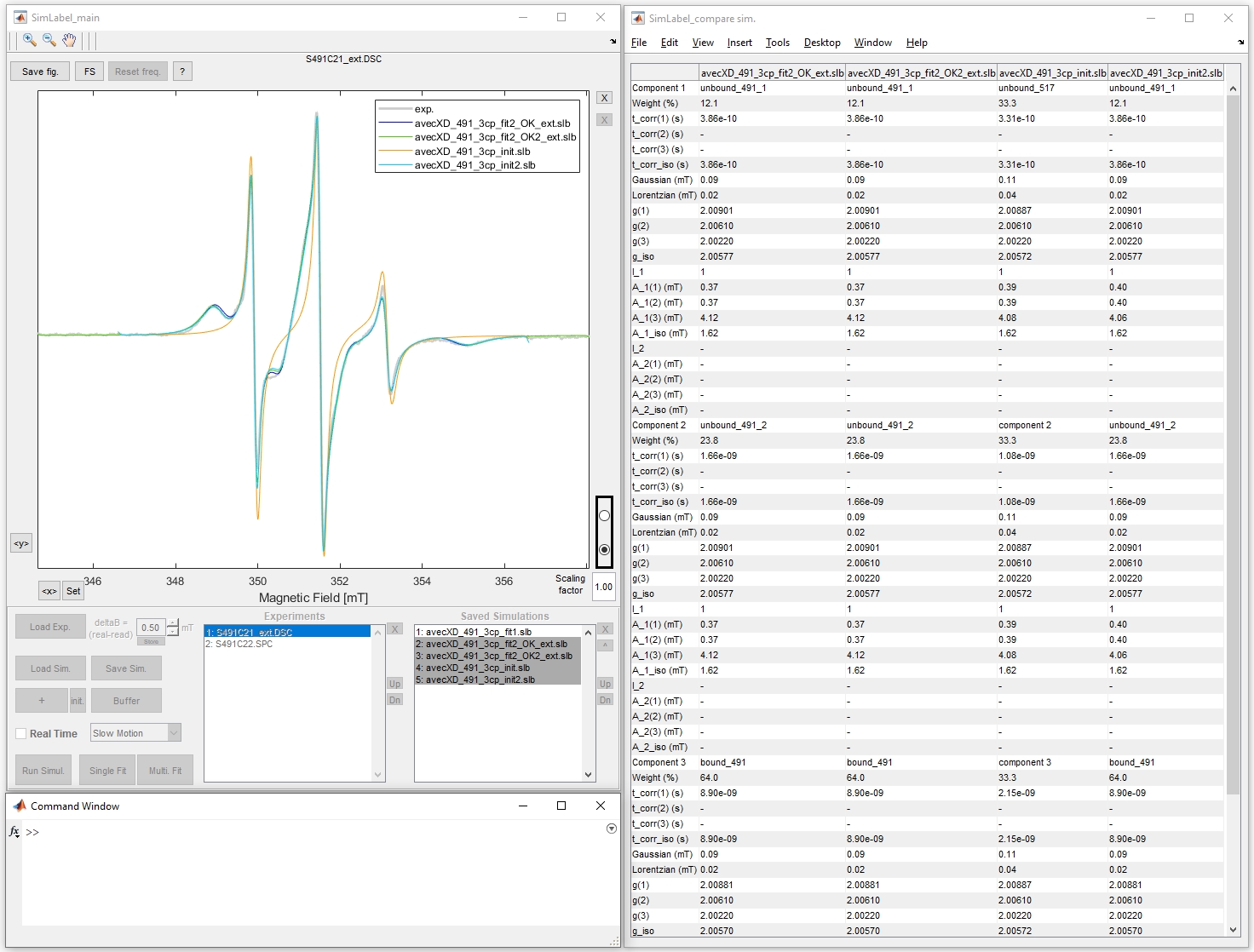
SimLabel is a Graphical User Interface (GUI). SimLabel provides an easy way, without coding, of visualizing, simulating and fitting continuous wave (cw) EPR spectra resulting especially from Site Directed Spin Labeling experiments.
SimLabel was first designed to facilitate the simulations of slow motion multicomponent nitroxide cw EPR spectra recorded at room temperature. Actually all the simulations of cw EPR spectra resulting from one unpaired electron (S=1/2), with small g-anisotropy, coupled to one or two nuclei with nuclear spins ranging from I=1/2 to 5/2, in the slow motion regime or in the solid state can be performed.
Bonus: use slbaverage to average several SimLabel simulations (*.slb files) and obtain uncertainties (confidence level 68%). The simulations to average must be « equivalent » (same simulation type, same component numbers, same parameters,…). The first selected .slb file is the reference. The average simulation is saved as a *.slb file. The uncertainties are saved as a pseudo-slb file (*_incert.slb). Download slbaverage.m and save it in a folder of the matlab path. To use it, whatever the current folder is, type in the matlab command window: slbaverage.
Version: SimLabel: Sept 2022 | slbaverage: 2018
See Also
Emilien Etienne, Nolwenn Le Breton, Marlène Martinho, Elisabetta Mileo, Valérie Belle. SimLabel: a graphical user interface to simulate continuous wave EPR spectra from site-directed spin labeling experiments. Magn. Reson. Chem., 2017, 55(8), 714 – 719.
DOI: 10.1002/mrc.4578HAL: hal-01444172v1
Emilien Etienne, Annalisa Pierro, Ketty C. Tamburrini, Alessio Bonucci, Elisabetta Mileo, Marlène Martinho, Valérie Belle. Guidelines for the Simulations of Nitroxide X-Band cw EPR Spectra from Site-Directed Spin Labeling Experiments Using SimLabel. Molecules, 2023, 28(3), 1348.
DOI: 10.3390/molecules28031348HAL: hal-03971418v1
These GUI scripts provide an easy way to automatically plot and adjusting kinetic from EPR spectra (1D or 2D), while controlling each spectrum processing. Data processing is kept in memory by saving and can be reloaded. The time associated to a spectrum is the time calculated for the middle point. Spectra are normalized by their scan number and amplitude modulation. Each spectrum can be selected by clicking its name in the list or by clicking its corresponding point on the kinetic curve.
kinetic.m extracts amplitudes of derivative, positive or negative lines, with denoising options (smoothing or SVD).
kinetic_intensity.m extracts intensity of each spectra with a polynomial baseline correction on absoprtion spectrum (numerical integration).
Download kinetic.m and/or kinetic_intensity.m and save it in a folder of the matlab path. To use it, place the spectra to analyse in a specific folder and choose it as the current folder, type in the matlab command window: kinetic or kinetic_intensity and follow the steps. If available, saved kinetic can be loaded when starting.
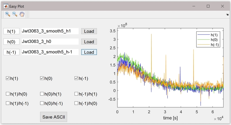
Bonus: visualize data generated by kinetic and kinetic_intensity with easyplot. Plot data ratio and save it as ASCII (*.txt). Download easyplot.m and save it in a folder of the matlab path. To use it, whatever the current folder is, type in the matlab command window: easyplot.
Version: kinetic: June 2020July 2021January 2022April 2023 March 2024 | kinetic_intensity: 2016Sept. 2020July 2021January 2022 March 2024 | easyplot: May 2020June 2021October 2023 March 2024
Extract_from2D
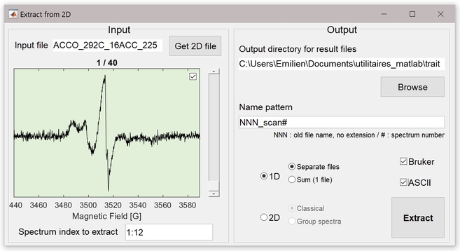
Extract_from2D extracts data from Bruker 2D experiments (*.DSC, *.DTA and *.YGF). The output data can be:
1D EPR spectra files in Bruker format (*.DSC and *.DTA) and/or ASCII (.txt). In this mode, the output can be separated spectra or one averaged spectrum.
2D EPR spectra files in Bruker format (*.DSC, *.DTA and *.YGF) and/or ASCII (.txt). In this mode, the « classical » output is a simple extraction of the primary data (whatever the selected indices), whereas the « Group spectra » output groups (sums) n by n spectra (n is specified by the user; the indices must follow each other).
The indices of spectra to extract can be given in the Matlab style (vector without [ ]) or by checking them one by one.
Download extract_from2D.m and save it in a folder of the matlab path. To use it, whatever the current folder is, type in the matlab command window: extract_from2D and follow the steps.
Version: May 2020Jul. 2020 Jan. 2021
Dataexp
Dataexp can convert 1D EPR Bruker files (*.DSC and *.DTA or *.SPC and *.PAR)
in ASCII files (*.txt or *.dat)
in figure (*.tif or *.fig).
Dataexp runs with single spectrum, spectra selection or all spectra of a directory.
Download dataexp.m and save it in a folder of the matlab path. To use it, whatever the current folder is, type in the matlab command window: dataexp.
Version: July 2020 May 2021
Saturation & Saturation_absorbtion
saturation
saturation_absorption
These GUI scripts provide an easy way to automatically plot and adjust saturation curve from EPR spectra (1D), while controlling each spectrum processing. Data processing is kept in memory by saving and can be reloaded. Spectra are normalized by their scan number, amplitude modulation and receiver gain. Each spectrum can be selected by clicking its name in the list or by clicking its corresponding point on the saturation curve.
saturation.m extracts amplitudes of derivative, positive or negative lines.
saturation_absorbtion.m extracts absorption (numerical integration) amplitudes of each spectra with a polynomial baseline correction.
Download saturation.m and/or saturation_absorbtion.m and save it in a folder of the matlab path. To use it, place the spectra to analyse in a specific folder and choose it as the current folder, type in the matlab command window: saturation or saturation_absorbtion and follow the steps. If available, saved saturation curve can be loaded when starting.
Version: 2016Jan. 2021June 2021January 2022 April 2023
Titration
This GUI script provides an easy way to automatically plot and adjust redox titration curve from EPR spectra (1D), while controlling each spectrum processing. Data processing is kept in memory by saving and can be reloaded. Spectra are normalized by their scan number, amplitude modulation, receiver gain and conversion time. Amplitudes of derivative, positive or negative lines can be extracted. Each spectrum can be selected by clicking its name in the list or by clicking its corresponding point on the titration curve.
Caution: the redox potential of each spectrum must be written in mV in the title string (case sensitive, lower-case « m » and upper-case « V »). This information must be written as in the following examples: ‘blablabla -320mV blablabla’ (no space between the number and mV, ‘+’ sign can be written or not, spaces before and after). If this information is missing or is not properly written, the spectrum is supposed to result from a « as prepared » sample.
Download titration.m and save it in a folder of the matlab path. To use it, place the spectra to analyse in a specific folder and choose it as the current folder, type in the matlab command window: titration and follow the steps. If available, saved titration curve can be loaded when starting.
Version: 2015Jan. 2021June 2021January 2022 April 2023
Checking Curie law
These GUI script provides an easy way to automatically plot and adjust A*T (Amplitude * Temperature (K)) as a function of temperature from EPR spectra (1D), while controlling each spectrum processing. Data processing is kept in memory by saving and can be reloaded. Spectra are normalized by their scan number, amplitude modulation, receiver gain, conversion time and power. Amplitudes of derivative, positive or negative lines can be extracted. Each spectrum can be selected by clicking its name in the list or by clicking its corresponding point on the curve.
Caution: the temperature of each spectrum must be written in kelvin in the title string. This information must be written as in the following examples: ‘blablabla 15K blablabla’ (no space between the number and K, spaces before and after).
Download checkcurie.m and save it in a folder of the matlab path. To use it, place the spectra to analyse in a specific folder and choose it as the current folder, type in the matlab command window: checkcurie and follow the steps. If available, saved processes can be loaded when starting.
Version: Jan. 2021June 2021January 2022 April 2023
Add g-scale
This GUI script enables to add chosen g values to *.fig spectra. The frequency can be picked up from experimental spectra (Bruker). The user can set the fontsize and the number of digits after the decimal point, and adjust the axe position.
Download addgscale.m and save it in a folder of the matlab path. To use it, whatever the current folder is, type in the matlab command window: addgscale.
Version: July 2020 August 2021
Magnetic field calibration
This GUI script enables to determine the magnetic field offset for a spectrum without any g-marker from a spectrum with g-marker. The spectrum with g-marker is corrected to consider the frequency shift. The calibration (ΔB=Breal – Bread) can be stored to be used in SimLabel.
Download deltaB_gmarker.m and save it in a folder of the matlab path. To use it, whatever the current folder is, type in the matlab command window: deltaB_gmarker.