QSoas

QSoas is a general-purpose data analysis program with particular strengths for the processing of $y = f(x)$ data, for massive data analysis (via the use of scripts) and for fitting, including massive fits.

This document gives you a general introduction about how to use QSoas. You can look at the documentation of each command in the command reference or at the FAQ.

You can use QSoas on Windows, Mac OSX and Linux, to:

• load and display $y = f(x)$ data from any ascii (text) file
• cut or concatenate datasets
• subtract various baselines
• remove noise
• fit datasets using arbitrary formulas, built-in functions or even the numerical solution of a kinetic system
• reparametrize fits
• fit using differential equations
• fit with parameter dispersion
• run global fits with shared parameters
• analyse the time evolution of a spectrum
• script operations that must be repeatedly run on numerous data sets
• and much, much more…

A step by step tutorial for QSoas

For this tutorial, you will need a series of example files. Download the following archive and unzip it.

Then start QSoas and take the time you need to go through all steps in this tutorial.

Start QSoas and change the current directory.

When you start QSoas on a computer running Windows, two windows will appear: a black text-window which you can ignore, the main window which looks like the image below, and a tips windows. On MacOSX and Linux computers, the black window will not be present.

In this window, locate:

• the tips window, which shows automatically at startup (but click on “Don’t show tips again” if you don’t want them);
• the list of menus (top left): File / Fits / View / Buffer / Simulations / Help;
• the graphic zone, which you can expand by dragging with the mouse a dot that is located just below the X at the bottom of this graphic zone. Sometime you can’t see the dot, just move your mouse around this zone until the handle appears;
• a large text-box, referred to as “QSoas’ terminal”, which shows, among other useful informations, the precise version and the location of the log file (here, C:/Users/Christina/soas.log):

Opening log file: C:/Users/Christina/soas.log
This is QSoas version 2.2.0+2020.05.19-release+r2683-817f303-qt5-newer-gsl running with mruby 1.3.0 and Qt 5.8.0
Built 2020-05-19 04:25:30 +0200 on 'nausicaa' with Qt 5.8.0 and GSL version 2.5
Copyright 2011 by Vincent Fourmond
          2012-2020 by CNRS/AMU

Based on Christophe Leger's original Soas
[...]
To get help on a specific command, type 'help command'

• a one-line text-box showng a prompt (QSoas>) and a blinking cursor. This is the command line, Linux style.

You will tell QSoas what to do by typing text in the command line. Commands can also be run trying to find things in the menus and clicking with the mouse, but we advise that you use the command line. A nice thing about clicking in the menus is that it shows you a dialog box with all the options available for the command.

For example, you can change directory by clicking on Menu/File/ChangeDirectory, then using the File Explorer (windows) or Finder (mac) to select the directory where you have unzipped the example files.

Alternatively, type either “G” or “cd” in the command line, and hit return. The File Explorer will open up for you to select the directory.

Finally, you can also select the new directory by typing the following text in the command line:

QSoas> cd E:/somewhere/QSoasExampleFiles (windows)
QSoas> cd /Users/me/somewhere/QSoasExampleFiles/ (mac)
QSoas> cd /home/somewhere/ (linux)

(then hit return). In this example, the command cd means “change directory”. QSoas will answer in the terminal: Current directory now is: E:/somewhere/QSoasExampleFiles. The name of the current directory is also written in the title bar above the list of menus.

When using a command from the menu, you can find its name either by looking at the status bar (below the prompt) or after you’ve run it, as it ends in the terminal as if you had typed it.

Loading a file.

Some commands can be run alone, others take arguments and/or options. E.g. in the command for changing directory above, cd is the command and the path name is an argument.

Let us load the example file file1.dat, by using the command load, followed by the argument file1.dat.

QSoas> load file1.dat

If the program answers in the terminal “Could not open 'file1.dat' for reading: No such file or directory”, this means you have forgotten to specify the current directory where the file is. Use the above command cd, or the menu File/Change directory, and try again.

Many QSoas commands can be called by using either a long name or a short name. For example to load a file, the long command load is equivalent to just the small letter L, l. Note that command names are case-sensitive. Try to run Load (with a capital L), and read the error message.

While you are editing a line of command, auto-completion is available with the tab key. It works so that when you write the first letter or letters of a command (or option or argument) and hit the tab key, the program predicts one or more possible completions as choices, and writes them either below the command line or in the terminal. Try it by typing l then hit the tab key.

Honestly, you should really get into the habit of using the tab key systematically. Beyond saving time, it also helps preventing spelling mistakes; most of the time, if QSoas cannot complete what you are typing, chances are it won’t understand it either.

Therefore, to load the file file1.dat, you may also type

QSoas> load file1.

and hit the tab key to auto-complete, try and see what happens.

Or you may just type load and return, or just l and return: a window will appear, for you to select the file you want to load.

Alternatively, you may use the comand browse (short name W):

QSoas> W

This opens a window showing all data files in the current directory, then tick the “select buffer” box that is just next to the file you want to load, then “push onto stack”, then “close”. Here you are.

QSoas> load file1.dat

After you have loaded the file, the window should look like this:

On the top left corner of the graphical window, you now see “file1.dat (#0)”. This is the name and number of the current data set.

You can use the upward and downward arrow of your keyboard to recall commands that you have used before, and the left/right arrow to re-edit a former line of commands, which will be very useful as you become an expert and your commands are more complex.

The stack

QSoas keeps the different data sets in a stack. These data sets are called buffers. The up-to-date buffer, usually displayed on screen, is number 0, hence “file1.dat (#0)”.

Modifying a buffer moves it upwards in the stack (then the former 0th buffer becomes number 1 etc…), while the new buffer takes position #0. This stack-based design permits to undo operations (with the undo command) by moving all buffers downwards, to redo what as been undone (with the redo command) by moving all buffers up in the stack. To pick a given buffer from the stack, use the fetch N command which copies buffer number #N to position number #0. You don’t need to understand this to use undo and redo, but you need to know that there is a stack to make the most of many advanced features of QSoas.

The command show-stack makes it possible to list the buffers. Let us create a few new buffers before we use it.

Select a fragment of a CV (cyclic voltammogram)

Imagine you want to analyze the oxidative part of the CV, you have to cut the data set first, use the command cut (or just c) and hit return, you get:

QSoas> c

The current is now plotted against “time” (actually, index = data point number) in the graphic window. The vertical dashed white lines mark the limits of the part of the data you will want to keep.

Examine the bottom-right part of the window, which lists the commands you can use at that point.

Change the left bound clicking with the left button at X=450. Change the right bound with a right click at X=800. Then “quit” clicking on the middle button (or typing q): you’re back with a new buffer where the parts outside the limits you selected have been deleted.

Run undo (or simply u) to get back to the complete CV, and try the commands splita and splitb (one at a time).

Note that the name of the buffer (shown on top of the graphic window) has changed. The name of the buffer will be automatically modified each time you run a command that modifies the data set. If you think that, at some point, the name of the current buffer has become too long, use the command rename with the name you want as an argument.

QSoas> rename new_buffer_name.dat

This does not affect the stack, only the name of the current buffer.

You may also cut the data using the strip-if command:

QSoas> strip-if ‘x < 100 || x > 520’

The above command will get rid of the data outside the interval $100 \leq x \leq 520$. The || bit means “or”.

Remove the noise

Use the command filter-fft to remove regular and/or high frequency noise from the voltammograms.

QSoas> filter-fft

The graphical window is now split in two. The upper window shows the raw data in red, and the smoothed data overlaid in purple. The difference (residuals) are plotted in black in the lower box. Examine the right part of the window, where there is a list of the actions that tune the filter.

To change the size of the cutoff, the easiest way is to display the power spectrum (PS) of the data = magnitude of the signal as a function of frequency. Type p, the lower box changes. The PS of the raw data now is plotted in red, that of the smoothed data overlaid in purple. The cutoff is indicated by a vertical dashed line in the PS. Click in the PS to adjust the cutoff. See the effect on the residuals by typing p to remove the PS and see the residuals.

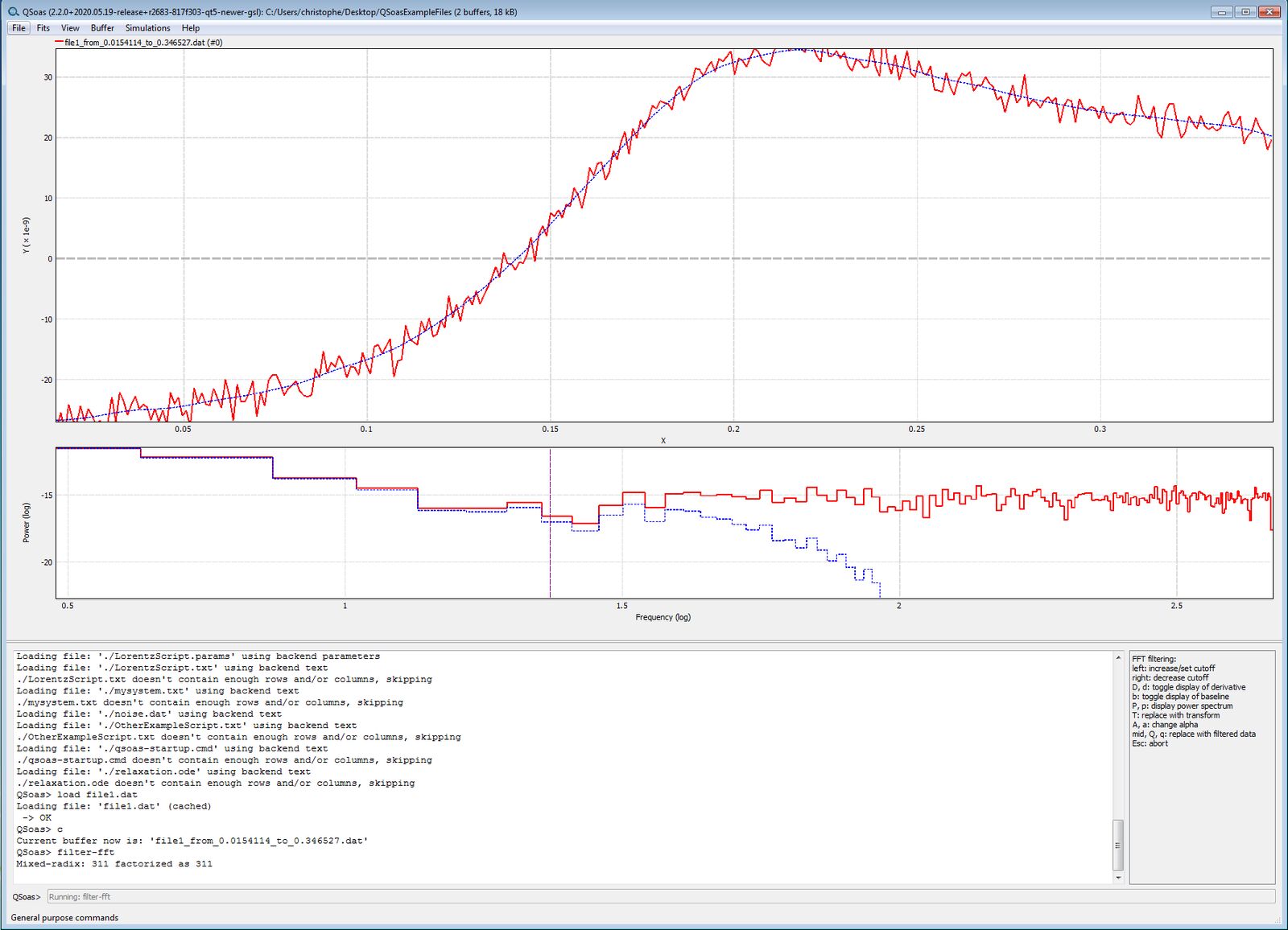
You want to make sure that the residuals are evenly distributed around Y=0, i.e. that you’re not over-filtering. When you are happy with the result, middle-click or type q. You get the smoothed data full screen.

Then run undo to get back to the noisy data, and try the following non-interactive command

QSoas> auto-filter-fft /cutoff=32

The command remove-spikes (short name R) takes no argument and does whatever it can.

The command deldp can also be used to remove spikes (to delete a data point that is significantly off, run deldp and click near the data point you want to remiove, quit by hitting q).

Subtract baselines

The reg command works just like cut, except that you should left/right click to define one segment that is used to fit a linear baseline (dotted blue). Try it.

QSoas> reg

You can move the bounds as many times as you want. When you are happy with your linear baseline, subtract it by typing u.

For many data, including spectroscopy and non-catalytic voltammetry with adsorbed species, you want to interpolate a baseline from the regions on either side of the peak(s) where the signal is zero. Like in SOAS, the QSoas command is baseline (or short: b). Interpolation uses a spline procedure. The markers that define the baseline are input clicking with the mouse. By typing s, x or o, the marker switches between Smooth, eXact or Off data. See the list of commands on the bottom right corner of the screen. Type q to quit, subtracting the baseline. Try it out with the file file5.dat:

QSoas> l file5.dat
QSoas> splitb
QSoas> b

The other baseline corrections available in SOAS are also available in QSoas using the following QSoas commands:

• catalytic-baseline (short name B) for a linear/polynomial/exponential baseline defined by two segments (four markers). (in both cases, b and B, you can either subtract the baseline or divide by the baseline)
• subtract (short name S) for subtracting a control signal.
• div for dividing by a control signal.

Get statistics about the current buffer

You can simply measure the main peak height & position. The non-interactive command 1 (the number one) looks for one extremum, and tells you in the text zone whether it is a maximum or a minimum, its X and Y values, the corresponding index, and the width at half-height when applicable. This information is saved in the file out.dat.

The interactive command cursor (shortname cu) makes it possible to click near a data point, whose coordinates (x,y,index) are output in the terminal. You can right-click to set a reference point, so that when you left-click to select another data point, you also get x-xr, y-yr, x/xr and y/yr.

The non-interactive command stats tells you everything you need to know about the current data set:

QSoas> l file1.dat
QSoas> splitb
QSoas> stats
Statistics on buffer: file1_b.dat:
x_sum =	 73.442993312	x_average =	 0.17444891523	x_var =	 0.0168957110344
x_stddev =	 0.129983502932	x_first =	 -0.0508118	x_last =	 0.398865
x_min =	 -0.0508118	x_max =	 0.398865	x_norm =	 4.4637590504
x_med =	 0.174561	x_q10 =	 -0.00595093	x_q25 =	 0.0624084
x_q75 =	 0.286713	x_q90 =	 0.354004	x_delta_min =	 0.001068
x_delta_max =	 0.00213623	
y_sum =	 1.727973303e-6	y_average =	 4.10444965083e-9	y_var =	 6.13300475277e-16
y_stddev =	 2.47649041039e-8	y_first =	 -3.95189e-8	y_last =	 2.27766e-8
y_min =	 -4.20774e-8	y_max =	 3.75436e-8	y_norm =	 5.15064927472e-7
y_int =	 1.82259238652e-9	y_med =	 1.84776e-8	y_q10 =	 -2.95887e-8
y_q25 =	 -2.26708e-8	y_q75 =	 2.52273e-8	y_q90 =	 3.16927e-8
y_delta_min =	 1.23e-11	y_delta_max =	 7.2873e-9	y_a =	 1.65901627747e-7
y_b =	 -2.48369093445e-8

Algebra

The command apply-formula can be used to transform your data. Examine the following examples:

QSoas> apply-formula x=x+0.241
QSoas> apply-formula x+=0.241
QSoas> apply-formula x,y=y,x
QSoas> apply-formula 'x=x+2 if (x>-0.3 and i>400)'

In the latter example, i is the index. In the latter example also, the quotes around the formula are necessary because it contains spaces.

You can use functions like abs(), log(), log10(), etc., and even special functions like bessel_j0() (see the full list here).

You can also use any output of the stats command in a formula. E.g. you can force y[0]=0 by running the following command:

QSoas> apply-formula y=y-$stats.y_first 

You even have automatic completion on $stats !

It may also be useful to use the command edit (which takes no argument) to see the X,Y table of values, and edit it.

Zoom

Point with the mouse somewhere in the graphical window near the data: you will see the coordinates of the nearest data point.

• Scrolling up/down with the mouse wheel will zoom in/out along the Y axis.
• Shift-scrolling with zoom along the X axis.
• Ctrl-scrolling (command-scrolling for mac users) will zoom in and out.
• Ctrl-Shift scroll will reset the zoom (command-shift-scroll if you use a mac).

You can also zoom in every individual window while you are using the command browse to select files in the current directory: just point the mouse in a small window and scroll.

If you like to have a rectangle to zoom, use the zoom command.

Save your data

To save a buffer into a text file on your hard drive, use the command save (short command s) followed by the filename of your choice as an argument, here process-file1.dat.

QSoas> s processed-file1.dat

Alternatively, you can omit the file name and have QSoas prompt you for one.

A header in the saved file has many lines of comments, normally starting with a #, that summarize the “history” of this buffer. In our example, saving the current buffer will produce a text file that starts like that:

# saved from Soas buffer name file1_from_-0.0273132_to_0.380707_filtered_linsub_mod_mod.dat
# commands = apply-formula x+=0.241
# apply-formula y,x=x,y
-1.86221e-10    0.213687
-2.12799e-10    0.214755
-2.40626e-10    0.215823
-2.69875e-10    0.216891
…

The stack is lost if you quit the program, unless you have saved it with the command save-stack (it can then be loaded with the command load-stack). There is no limit to the size of the stack (but QSoas will have a hard time with stacks larger than your computer’s memory, which should not happen often anyway).

See the content of the stack

You can list the buffers in the text-box by running the command show-stack (short name: k). You will see in the terminal a series of lines like this:

QSoas> k
Normal stack:
    F    C    Rows   Segs
#0       2    382    1    "E:/PrivateFolder/QSoasExampleFiles/file1_from_(…).dat”    
#1       2    382    1    "file1_from_(…).dat    
(…)
#5       2    382    1    file1.dat    

• The 1st column is the buffer number, which is positive for the normal (undo) stack and negative for the redo stack.
• The 2nd column (F) has a star if the buffer is “flagged”. Flagging makes it easier to select a series of buffers (see below).
• The 3rd column (C) indicates the number of columns in your buffer (at least 2, sometimes more).
• The 4th column (Rows) indicates the number of data points.
• The 5th column (Segs) indicates the number of segments.
• The last column indicates the name of the buffer.

Define your first alias

If the stack is too large, you can see a shorter list by typing

QSoas> show-stack /number=10

If you always use the above command, you may define a new, shorter command (say, “k10”) which will do the same thing:

QSoas> define-alias k10 show-stack /number=10

Plot/print several buffers at once, and (un)flag them.

To overlay several data sets (for the sake of comparison), you can use the commands overlay (short name lower case v), which will load a file and plot it together with buffer #0. For example:

QSoas> overlay *.dat

will load and plot on top of buffer #0 all files in the current directory whose name ends with .dat

The command overlay-buffer (short name capital V) is followed by a list of buffer numbers. For example:

QSoas> overlay-buffer 1,8..10,15..19:2

will plot buffers 0, 1, 8, 9, 10, 15, 17, 19. NB: we use “..” rather than “-“, else there is an ambiguity with the minus sign of the buffers in the redo stack.

You can flag buffers and then plot all flagged buffers on top of buffer #0 using this sort of commands:

QSoas> flag 1,8..10
QSoas> flag 15..21:2
QSoas> unflag 21
QSoas> overlay-buffer flagged

To unflag everything, run:

QSoas> unflag flagged

If you’are happy with the result and want to print it, try the command

QSoas> print /file=filename.pdf /title=text

Without the option /file=, the plot will be sent to the default printer, rather than saved as a pdf file on the hard drive.

Fits

A simple example with one data-set, one equation, one set of parameters.

Imagine you have run a titration experiment, whose result (intensity against potential) is in file2.dat, and you want to fit a sigmoid to these data points.

One way to do it, is to load the file, then use the command fit-arb that allows you to fit using a user-defined function to the current buffer.

QSoas> fit-arb a/(1+exp(96500/8.31/temperature*(x-e0)))

where the argument is the function you want to use. It must depend on x, all other combinations of letters are interpreted as parameters (here: a, temperature and e0). A parameter name cannot start with a capital letter.

A series of physical constants are available (they start with an uppercase letter): F (Faraday constant), R (the gas constant) and PI. A full list is available in the documentation. Therefore, it does the same to run:

QSoas> fit-arb a/(1+exp(F/R/temperature*(x-e0)))

As QSoas was born in the electrochemistry world, there is a special shortcut for F/R/temperature, named fara. Hence, the above fit could have been written thus:

QSoas> l file2.dat
QSoas> fit-arb a/(1+exp(fara*(x-e0)))

When you run the fit-arb command, a new window opens up, which shows

• the data set (red) and the fit (green) in the main graphic box,
• the residual in the lower graphic box,
• the equation of the fit,
• the list of parameters, each with a text box where you can set or read their values, followed by a smaller box which you can tick to “fix” a parameter (if you do not want the program to adjust it).
• a series of “actions”, which you can execute from 3 menus and 4 buttons: Data… / Parameters… / Print… / Update Curves (Ctrl U) / Edit parameters (Ctrl E) / Fit (Ctrl F) / Close (Ctrl W). If you are using a mac, it is Cmd, not Ctrl.
• a selector for the Fit engine.

Set the initial guess by inputting reasonable values for a (e.g. 1.5) and e0 (e.g. 0.3). Check your initial guess by hitting the “Update curves” button (or Ctrl U), then hit the “fit” button (or just type Ctrl F)

The best values of the parameters are now written in the text boxes, on a green background, because the program thinks they are well defined. You can see the covariance matrix of the parameters in the “Actions/Parameters…” list of actions (or just type Ctrl M). From the same menu, you can save the parameters in a file (e.g. file2.params) that you will want to use again later. Or just type Ctrl S.

You need to use Actions/Data…/Push Current to Stack before you close the window (Ctrl W) if you want to get the best fit into a buffer, which you can save on disk.

Rerun the fit and see the effect of ticking “(fixed)” after a parameter.

You may also want to force a parameter to belong to a certain interval. Click on “Edit parameters” (bottom right), then select “Range (hyperbolic)” and enter the limits of the interval.

If you don’t want to type a complex equation too often, you may prefer to write it once in a file then load it. Open a text editor and examine the content of the file exampleFitFunctions.txt. It has the following lines:

sigmoid: a/(1+exp(F/R/temperature*(x-e0)))
line: a*x+b

which define new functions that can be used for fitting. Load this file by typing

QSoas> load-fits exampleFitFunctions.txt

The above command creates three new commands, fit-sigmoid, mfit-sigmoid, and sim-sigmoid, which will all be forgotten after you quit QSoas.

Since you have previously saved the best parameters in a file, e.g. file2.params, you can directly run

QSoas> fit-sigmoid /parameters=file2.params

to use as an initial guess the former best parameters.

Combining functions

Examine the following example

QSoas> load-fits exampleFitFunctions.txt
QSoas> l file2.dat
QSoas> apply-formula y=y+2*x
Applying formula 'y=y+2*x' to buffer file2.dat
Current buffer now is: 'file2_mod.dat'
QSoas> combine-fits mynewfit 'y1 + y2' sigmoid line
QSoas> fit-mynewfit

The first command loads file2.dat.

The second command modifies the data by adding a linear trend.

The command combine-fits creates a new command, fit-mynewfit, which will fit data to a sum of two functions, sigmoid and line; these functions were previously defined when we loaded exampleFitFunctions.txt.

The command fit-mynewfit runs the combined fit on the modified data-set.

Advanced fit: two data sets, one model, two sets of parameters.

Imagine you have performed a redox titration by measuring an intensity as a function of potential at two wavelengths, or whatever, and the results are in file2.dat and file3.dat. You can use QSoas to fit an equation to the two data sets at once.

Load file2.dat, then file3.dat, so that file2 is in buffer #1 and file3 in buffer #0. See what the data look like.

QSoas> l file2.dat file3.dat

We need an equation that could apply to both data sets. The example file exampleFitFunctions.txt also contains the following line:

general-sigmoid: a/(1+exp(F/R/temperature*(x-e0)))+b

and therefore the command load-fits exampleFitFunctions.txt has also created three new commands called fit-general-sigmoid, mfit-general-sigmoid and sim-general-sigmoid.

To fit multiple data-sets at once, the command is called mfit-something, followed by the numbers that identify the buffers. So here, we shall use

QSoas> load-fits exampleFitFunctions.txt
QSoas> mfit-general-sigmoid 0 1

The fit window opens up. It looks the same as before except that now:

• you can use the horizontal arrows on either side to see the different data sets and the corresponding best fits.
• each parameter can be fixed to a certain value and/or global (meaning that it must have the same values for all data sets).

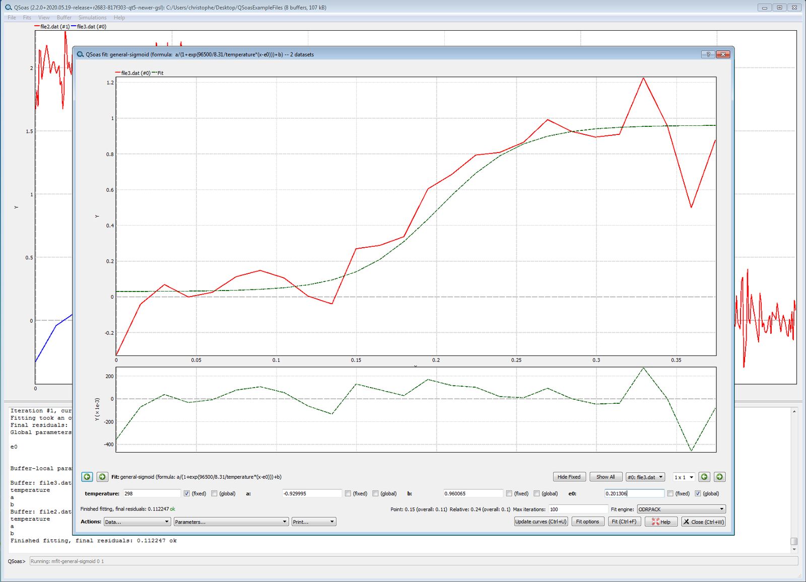
Set e0 to 0.3, and for this parameter, tick “fixed” and “global”, then run the fit (Ctrl F). See what has happened by clicking on the horizontal arrows.

Set e0 free by unticking the “fixed” box. Ctrl F. See the results.

Save the parameters into a file (Ctrl S), e.g. file2-file3.params. Close.

If you want to give more weigth to one of the two data sets, run:

QSoas> mfit-general-sigmoid 0 1 /parameters=file2-file3.params /weight-buffers=true

Now there is an other box, called “weight” which you can change for each data set. Give file3.dat a large weight and run the fit.

The same, but differently.

The same operation can be run in a different manner, by making use of “segments” that define different parts in the same buffer, and having an equation that is segment-dependent. Let us combine file2 and file3 in the same buffer. Load file3.dat, then file2.dat, so that file3 is in buffer #1 and file2 in buffer #0, then concatenate the two data sets using the command i (short for cat), and run show-stack to check that the current buffer is made of 634 points, and has two segments.

QSoas> delstack
QSoas> load file3.dat
QSoas> load file2.dat
QSoas> i 0 1
QSoas> show-stack
Normal stack
      F    C    Rows    Segs
#0         2    634     2    file2_file3.dat
#1         2    608     1    file2.dat
#2         2    26      1    file3.dat

If a data set is made of two segments, the first segment is 0, the second segment is 1. The segment number can be used in a formula. E.g.:

QSoas> apply-formula "y=2*y if seg==1"

Now run the following command

QSoas> fit-arb (1-seg)*a1/(1+exp(fara*(x-e0)))+seg*a2/(1+exp(fara*(e0-x)))

Set a reasonable guess for the value of e0 before you hit “Fit”.

More advanced fit: one data set and its derivative, a single set of parameters

To increase the reliability of the parameters, it may be useful to fit a model to a data set and the first derivative of the data set.

Let us illustrate this with file2.dat. Load the file, then run

QSoas> filter-fft /derive=1

Show the power spectrum (by hitting p) and select a cutoff of about 23, then quit to get into buffer #0 something that resembles a derivative of a sigmoid, while file2 is now in buffer #1.

Alternatively, just run

QSoas> auto-filter-fft /cutoff=23 /derive=1

To run the fit with both data sets, let us first create a new command:

QSoas> define-derived-fit sigmoid

Then run the new command on the derivative of the data (in buffer #0) and the raw data (in buffer #1):

QSoas> mfit-deriv-sigmoid 1 0 /parameters=file2-file3.params

Even more advanced fit: two data sets, two models, one set of parameters.

Let us repeat the same analysis (data+derivative) but completely differently, to illustrate another possible method.

The file ExampleRubyFunctions.rb contains the following lines, which define two functions:

def sigmoid(a,temperature,x,e0)
 return a/(1+exp(fara*(x-e0)))
end
def sigmoidderivative(a,temperature,x,e0)
 return -a*fara*exp(fara*(x-e0))/(1+exp(fara*(x-e0)))**2
end

Load the ruby file by running

QSoas> ruby-run exampleRubyFunctions.rb

This does not create new commands; rather, it defines new functions, which can be used as arguments for the commands fit-arb and mfit-arb. If we want to fit the sigmoid and its derivative to the data set (buffer #1) and its derivative (buffer #0), run:

QSoas> mfit-arb sigmoid(alpha,temperature,x,e00)|sigmoidderivative(alpha,temperature,x,e00) 1 0 /parameters=file2.param

Note that the name of the parameters need not be the same in the above call and in the ruby file: only the position of the parameter matters. You can fit with as many functions and buffers at a time as you want.

The ruby syntax can be more sophisticated, as exemplified below:

def gas_injection(t, t0, c0, tau)
 if t < t0
  return 0
 else
  return c0 * exp(-(t – t0)/tau)
 end
end

Forcing relations between parameters of the model(s).

Imagine you want to analyse a 1st order relaxation (forward rate constant k1, backward rate constant k2, equilibrium constant k=k2/k1). You may want to fit an experimental exponential decay with

QSoas> fit-arb (k1/(k1+k2)*exp(-x *(k1+k2))+k2/(k1+k2))

Then you may realize that k2/k1 is better defined than k1 and k2, and that it would have make more sense to write the equation as a function of, say, k1 and k, instead of k1 and k2. Run the following command:

QSoas> fit-arb (k1/(k1+k2)*exp(-x*(k1+k2))+k2/(k1+k2)) /extra-parameters=k

and fix k2 to “=k*k1”. You may either fix k, or let the program adjust it.

Having an extra parameter may also be useful if you are fitting several models to several data sets, and want to impose a relation between the parameters of two distinct models.

Using built-in fitting functions

Many fit-, mfit-, and sim- commands are built-in. They can be used to fit exponential decays, peaks, Nernstian sigmoids, or electrochemical data, as described in the section about fits in the manual.

For example, the command fit-adsorbed can be used for fitting Nernstian peaks to non-catalytic voltammetric signals for adsorbed species.

The option /species= gives the number of peaks. The option /distinct=true allows the peak to have different areas.

QSoas> fit-adsorbed /species=2 /distinct=true

Here is the result of the fit of the backward sweep of file5.dat, setting n=1 for the two peaks, but the values of Gamma are free.

Here is another fit of the same data set, where the two values of $n$ are free and the two values of $\Gamma$ are forced to be identical (see Gamma_1=Gamma_0 and the “fixed” box ticked)

Other example, the fit-lorentzian command fits a lorentzian function (or a sum of lorentzian functions) to a signal. The following list of commands loads two spectra, and fits a sum of two Lorentzian functions to the two data sets, making sure that the peaks have the same positions and widths for the two data sets, but different amplitudes.

QSoas> load file4.txt
Loading file: './file4.txt' using backend text
 -> OK
QSoas> load file5.txt
Loading file: './file5.txt' using backend text
 -> OK
QSoas> mfit-lorentzian 0 1 /number=4 /parameters=file4-file5.params
Loaded fit parameters from file file4-file5.params

Before running the fit, the parameters can been edited (CTRL+E) to force the amplitudes and positions to be positive (set up transformation: log).

Here is the result:

Fit one or several data set(s) using the numerical solution of a kinetic system

Imagine you are trying to analyze the change in a signal which is proportional to the concentration of a species A that disappears according to $dA/dt=-k A$. If the initial concentration of A equates 1, the initial concentration of B is 0 and k=0.5, then the data should look like the buffer generated using the following command,

QSoas> generate-dataset .01 10 /samples=100 exp(-0.5*x)+0.01*sin(100*x)

where the sin() function is added to simulate some noise.

You can simulate the data using the numerical solution of a kinetic system that is defined in the file mysystem.txt, included in the ExampleFile directory:

A->B[k] 

To fit the model to the data, run

QSoas> fit-kinetic-system mysystem.txt

The program opens the fit window where one can see 5 parameters: y_A and y_B: the program assumes that the Y data is a linear combination of the instant concentrations of A and B: Y=Y_A*[A]+Y_B*[B]. c0_A and c0_B, the initial concentrations of A and B k: the rate constant

If the data set corresponds to the concentration of A, then fix y_A to 1, y_B to 0, c0_A to 1 and c0_B to 0 and hit “fit”. Here you are, k=0.5.

Other kinetic systems may be defined, using this sort of syntax:

# 2nd order, irreversible transformation of A into B with the 2nd order rate constant k1, so that dA/dt=-2*k*A**2
A+A->B[k]
# 1st order, reversible conversion between A and B, dA/dt=-k1*A+k2*B
A<=>B[k1][k2]
# pseudo 1st order transformation of A into C
A+B<=>C[k1/c_B][k2]

More complex schemes will be described in a text file that contains several lines

E+S<=>ES[k1][k2]
ES->E+P[k3]

The command mfit-kinetic-system can be used to analyze several data sets at once.

How to reparametrize fits, more advanced example

Let’s have a look at file6.dat, in which is recorded the concentration of a species A that evolves over time according to:

$$A \stackrel{k_i, k_a}{\rightleftharpoons} B$$

in which $k_{i}$ is the forward rate constant and $k_{a}$ the backward rate constant. In that case, and assuming that the initial concentration of I is 0, the time evolution of the concentration of A follows the equation:

$$A(t) = A_0\left(1 - \frac{k_a}{k_i + k_a}\right)\exp(-(k_a + k_i) t) + A_0\frac{k_a}{k_i +k_a}$$

The time evolution can be fit with a mono-exponential decay, but it may be more useful to reparametrize it to have the $k_{i}$ and $k_{a}$ explicitly as fit parameters. The equation for the mono-exponential fit is (see the manual):

$$A_\infty + A_1 \exp(-(x - x_0)/\tau_1)$$

Identification with the other equations gives the following relations:

$\tau_1 = \frac{1}{k_a + k_i}$ $A_\infty = A_0 \frac{k_a}{k_a + k_i}$ $A_1 = A_0 \frac{k_i}{k_a + k_i}$

To reparametrize, launch the following commands:

QSoas> l file6.dat
QSoas> fit-exponential-decay /extra-parameters=A_0,k_i,k_a

The /extra-parameters=A_0,k_i,k_a bit adds other named parameters to the fit, which we will use to reparametrize the fit.

Now load the file6.params parameters. You see that A_inf, tau_1 and A_1 are fixed, with formulas. To do that just fix the parameter, and use a formula starting with = as the parameter value. Now just run the fit ! You’ll see that the new parameters A_0, k_i and k_a have been adjusted.

Of course, in that specific case, it would have been simpler to define a kinetic system with the following file:

A <=> I [k_i][k_a] 

How to fit ordinary differential equations to data

The above problem can also be solved by writing the differential equations and integrating them. The equations take the form:

$\frac{\mathrm{d}c_A}{\mathrm{d} t} = k_a c_I - k_i c_A$ $\frac{\mathrm{d}c_I}{\mathrm{d} t} = - k_a c_I + k_i c_A$ $c_I(t = 0) = 0$ $c_A(t = 0) = c_{A0}$

These equations translate into the following file, named relaxation.ode:

c_A = c_A0
c_I = 0

d_c_A = k_a * c_I - k_i * c_A
d_c_I = - d_c_A

The blank line separates the initial conditions from the expression of the derivatives. QSoas automatically detects the parameters. Note that, like in all ruby code, you should refrain from using parameters that start with an UPPERCASE, as it confuses the Ruby interpreter (for Ruby, names starting with an uppercase are constants, and therefore cannot be parameters).

Now proceed as follows:

QSoas> l file6.dat
QSoas> fit-ode relataxion.ode

Your fit dialog box should look like this:

Note that by default, QSoas fits a linear combination of the integrated functions to the data; the coefficients are visible here as y_c_A and y_c_I (the coefficients are all set to 0 and fixed but for the first one). Don’t forget to fix either y_c_A or c_A0 before fitting: the computed curve is proportional to their product, which means that they of course cannot be determined independently. Not doing so will result in a fit that does not converge.

If what you need to fit is a more complicated function of the integrated functions, you can add a third stanza to the ODE definition, like in relaxation-2.ode:

c_A = c_A0
c_I = 0

d_c_A = k_a * c_I - k_i * c_A
d_c_I = - d_c_A

c_A * i_A

In that case, the fitted function is just i_A times the value of c_A (the concentration of A). Note that in this case, you still need to fix either c_A0 or i_A.

QSoas> fit-ode relataxion-2.ode

You can of course use much more complicated equations.

Dispersion of parameters

Sometimes, a model does not fit the data very well because the data is the sum of a large number of slightly different responses, for instance if it results from from a large number of molecules whose properties are slightly different.

Dispersion example 1: exponential relaxation

Let’s first assume that a process of some kind gives an exponential relaxation whose time constant is uniformly distributed over an interval, such as what is in file7.dat. Let’s first check that the fit using a normal exponential decay is poor:

QSoas> l file7.dat
QSoas> fit-exponential-decay

To fit this with a uniform distribution of relaxation time constants, run:

QSoas> define-distribution-fit dist-exp exponential-decay tau_1 /distribution=uniform
QSoas> fit-dist-exp

Now, one can see that the fit is much better, in particular at the beginning of the relaxation, where the uniform dispersion is expected to make a significant difference.

Dispersion Example 2: distribution of orientation of redox-active enzymes

Another case in which microscopic parameters are distributed that is the dispersion of electron-transfer rates in protein film voltammetry (see for instance Leger, et al, J. Phys. Chem. B 2002). For the sake of simplicity, let’s assume a one-electron reduction with potential $E_0$ and interfacial rate constant $k_0$ couple with a catalytic reaction of rate $k_2$ (for the reduced species). It is easy to demonstrate in this case that the catalytic current is proportional to:

$$i = \frac{i_{max}}{1 + \frac{k_2}{k_0} \exp \frac{F(E - E_0)}{2\,RT} + \exp \frac{F(E - E_0)}{RT}}$$

Data can be fit to this model by defining the following custom fit:

QSoas> custom-fit 1el 'imax/(1 + k2_ov_k0 * exp(fara * 0.5*(x - e0)) + exp(fara * (x - e0)))'

Note that there is no point to define both a k0 and a k2 parameter here, as only their ratio has an influence on the value of the current, which means that they cannot be determined independently.

Now try to fit the contents of file8.dat using that fit:

QSoas> l file8.dat
QSoas> fit-1el /parameters=file8.1el.params

As you can see, the fit is decent, but not perfect. This is due to the fact that there is a dispersion of values of $k_0$ (and hence of the values of the parameter k2_ov_k0). To fit that, we’ll define another fit using define-distribution-fit

QSoas> define-distribution-fit 1el-distrib 1el k2_ov_k0 /distribution=k0

The /distribution=k0 means that the the value of k2_ov_k0 is distributed so that its log value is uniform in the range $\log(max) \geq \log(k) \geq \log(max)/(\beta d_0)$. And then, we’ll fit using

QSoas> l file8.dat
QSoas> fit-1el-distrib /parameters=file8.1el-distrib.params

See that the k2_ov_k0 parameter has been replaced by k2_ov_k0_max and k2_ov_k0_betadmax, that correspond respectively to the highest value of k2_ov_k0 and the maximum value of $\beta d_0$. Be warned, though, that integrating over a distribution of parameters is computationally quite expensive, and will typically take 10 to 100 times longer to fit than the corresponding plain fit. There are other distribution types than k0 (gaussian, lorentzian, uniform), check the documentation of define-distribution-fit for more information.

A full example: fitting the evolution of spectra in time

Many kinetic techniques record the evolution of the spectrum of a sample as a function of time. QSoas makes it easy to fit those to extract the different components. It works using the capacities of multi-fit mentioned above. One first converts the spectra for different times into time evolution of the absorbance for different wavelengths, and then one fits all the time evolution traces together using whatever model is appropriate. The kinetic parameters (rate constants or time constants) have to be common to all the time traces, but on the contrary, the parameters related to the spectral components, such as the amplitude of exponential phases, change at each wavelength.

The data used for this tutorial were kindly given by Frauke Baymann and Fabrice Rappaport. They come from the study of photosynthetic reaction centers (Baymann and Rappaport, Biochemistry 1998). These spectra were recorded using a Joliot spectrometer, but the method shown below is applicable to all the techniques which acquire series of spectra for different times (or different potentials, for instance, in the case of a redox titration), such as those coming from freeze-quench or stopped-flow experiments.

The sample data being in the Joliot/ subdirectory, let’s first load all the spectra in one go using the following command:

QSoas> l Joliot/*.dat
QSoas> k
Normal stack:
     F  C   Rows    Segs
#0      2   17  1   'Joliot/spectrum-09.dat'
#1      2   17  1   'Joliot/spectrum-08.dat'
#2      2   17  1   'Joliot/spectrum-07.dat'
#3      2   17  1   'Joliot/spectrum-06.dat'
#4      2   17  1   'Joliot/spectrum-05.dat'
#5      2   17  1   'Joliot/spectrum-04.dat'
#6      2   17  1   'Joliot/spectrum-03.dat'
#7      2   17  1   'Joliot/spectrum-02.dat'
#8      2   17  1   'Joliot/spectrum-01.dat'
#9      2   17  1   'Joliot/spectrum-00.dat'

The first task is to convert the data into something that we want to fit. We need to convert a series of spectra for different value of the time, into a series of time evolution of absorbance for different wavelength. This goal is achieved in four steps, as detailed below. First, let’s gather all the data into a single dataset with as many Y columns as there are different times, using contract:

QSoas> contract 9..0

This creates a 11-column buffer with one X column (the wavelengths) and 10 Y columns (the absorbances at different times). The buffer list order is reversed 9..0 so that spectrum 00 ends up being the first column.

Now, we need to indicate the time that corresponds to each of the Y column. This is called the “perpendicular coordinate” in QSoas’s terminology. Setting the perpendicular coordinate is done via the set-perp command:

QSoas> set-perp 4e-05,0.0001,0.0002,0.0005,0.001,0.002,0.004,0.008,0.015,0.03

That the correct perpendicular coordinates were given can be checked using the command show

QSoas> show 0
Dataset Joliot/spectrum-00_cont_Joliot/spectrum-01_cont_Joliot/spectrum-02_cont_Joliot/spectrum-03_cont_Joliot/spectrum-04_cont_Joliot/spectrum-05_cont_Joliot/spectrum-06_cont_Joliot/spectrum-07_cont_Joliot/spectrum-08_cont_Joliot/spectrum-09.dat: 11 cols, 17 rows, 1 segments
Flags: 
Meta-data:  file-date = 2014-10-06T15:56:30 original-file = /home/fv/tmp/qst/QSoasExampleFiles/Joliot/spectrum-00.dat   age = 1625.49
    time = 4e-05    Perpendicular coordinates: 4e-05, 0.0001, 0.0002, 0.0005, 0.001, 0.002, 0.004, 0.008, 0.015, 0.03

Now, we convert this “series of spectra for different times” dataset into a “series of time evolution of absorbance for different wavelengths”. This is done using the command transpose (it is indeed a matrix transposition).

QSoas> transpose
QSoas> show 0
Dataset Joliot/spectrum-00_cont_Joliot/spectrum-01_cont_Joliot/spectrum-02_cont_Joliot/spectrum-03_cont_Joliot/spectrum-04_cont_Joliot/spectrum-05_cont_Joliot/spectrum-06_cont_Joliot/spectrum-07_cont_Joliot/spectrum-08_cont_Joliot/spectrum-09_transposed.dat: 18 cols, 10 rows, 1 segments
Flags: 
Meta-data:  file-date = 2014-10-06T15:56:30 original-file = /home/fv/tmp/qst/QSoasExampleFiles/Joliot/spectrum-00.dat   age = 1625.49
    time = 4e-05    Perpendicular coordinates: 580, 570, 565, 562, 561, 560, 559, 558, 557, 556, 555, 554, 552, 550, 548, 545, 540

As can be seen above, what were the usual coordinates before (the wavelengths) have now become the perpendicular coordinates. We still need to separate that buffer into many X,Y buffer that can be fit:

QSoas> expand /flags=joliot

The /flags=joliot tells QSoas to add the flag joliot to all the datasets created this way. We have completed the first part of the data analysis, which is to put the acquired data in a form that can be fitted.

To go any further now, we have to imagine a model that would fit the data. First, with the knowledge that the reactions whose kinetics we are now studying are purely first order, we know that the time evolution of the absorbance at any wavelength will be multi-exponential. Like in the original paper, we will fit the time evolution of absorbance with a bi-exponential decay:

$$A_\lambda(t) = A_{\lambda,\infty} + A_{\lambda,1} \exp(-t/\tau_1) + A_{\lambda,2} \exp(-t/\tau_2)$$

Note that, while the amplitude of each phase is different for each wavelength, the time constants $\tau_1$ and $\tau_2$ are the same for all wavelengths. The $A_{\lambda,1}$ and $A_{\lambda,2}$ correspond to the amplitudes of the first and second phase at a given wavelength, while $A_{\lambda,\infty}$ is the absorption spectra at infinite time.

Fitting the above formula to the data can be done using the following command:

QSoas> mfit-exponential-decay /exponentials=2 flagged:joliot

Your screen should look like that:

Note that the value of the perpendicular coordinate (here the wavelength) is shown next to the name of the buffer: Z = 540. We impose that tau_1 and tau_2 are common to all buffers. We also set x0 to 0 for all the buffers, though in practice this will not affect the determined times, and have very little effect on the amplitudes.

Next, we fit, by clicking on the Fit button. To get a better view of the overall fit, we can use the dropdown menu next to the arrows on the right hand side (it initially shows 1x1).

QSoas has two visualization features that make it easy to work with perpendicular coordinates. First, it is possible to display the parameters as a function of the perpendicular coordinates, which gives the spectrum for the different exponential phases and the final spectrum. For that, click on the “Show parameters” option from the “Parameters” menu, and select all the amplitudes through the check boxes:

From that window, it is possible to push these spectra to the stack using the “Push visible” or “Push all” buttons. See how these spectra are similar to the ones from figure 3 of the original paper.

Second, it is possible to show the original spectra for different times (ie the data before transposition) together with the fit. This is important, as it shows artifacts that may not be obvious from the other view (such as data at a given time that is systematically not fitted correctly, which is hard to spot from the time view). To access to that, just select the “Show transposed data” item from the “Data” menu.

Not all the kinetic experiments can be fit by sums of exponentials. The approach described above is absolutely not limited to mfit-exponential-decay fit. Indeed, any fit can be used. The one that will probably be the most useful to interpret kinetic data of this kind is the kinetic-system we described above. For instance, we could also interpret the data using an oversimplified model such as this one (available in the data files under the name Joliot.txt):

A -> C [k_fast]
B -> C [k_slow]

Fitting this model to the data is just a matter of running

QSoas> mfit-kinetic-system Joliot.txt flagged:joliot

For each buffer, the evolution of the concentration of the A, B and C are computed from the kinetic system shown above. The y value fitted to the data is a linear combination of the concentration, each multiplied by the corresponding y_ parameter (one of y_A, y_B and y_C). For this specific setup, the y_ parameters are therefore proportional to the extinction coefficients of the different species. The y_ parameters should be therefore free and buffer-specific (as they depend on the wavelength). While this is already the case for the y_A parameter, this is not the case for the y_B and y_C parameters. The simplest way to change that is to untick the “Fixed” box, set to a non-zero initial value, such as 1000 and then, click on global, and click on global again. This last step has for effect to copy the current parameter to all the buffers. The initial value should be non-zero (and of the correct order of magnitude), as fit engines work with relative variations. Then we’ll assume that the initial concentration of A and B are 1, edit that (and click on the global checkbox to make sure the initial concentration is the same for all buffers). The last thing before fitting is setting the k_fast and k_slow parameters to reasonable values, such as 1e4 and 1e3 respectively, and make sure they are global.

Then, all that’s left to do is to fit ! As before you can also look at the spectrum of species A, B and C using the “Show parameters” menu item.

One of the particularly attrative possibilities of using the kinetic-system fit is that it is not limited to first-order reactions, which is particularly important for simulating data coming from stopped-flow experiments.

Scripts

A script is a text file that contains a list of commands, which you can execute using the command run (short name: @). Comments in the script are indicated by the hash symbol. Examine the file ExampleScript.txt which reads

load file2.dat
auto-filter-fft /cutoff=23 /derive=1
ruby-run exampleRubyFunctions.rb
mfit-arb sigmoid(a,temperature,x,e0)|sigmoidderivative(a,temperature,x,e0) 1 0 /parameters=file2.param

Now run:

QSoas> @ ExampleScript.txt

If the above command is followed by arguments, they will replace the expressions ${1}, ${2} etc. in the script file. If you want to use a list of files or buffer as an argument and execute the script for each data set, use the command run-for-each. For example, try OtherExampleScript.txt, which reads:

load ${1}
splita
auto-filter-fft /cutoff=23 /derive=1
flag

and run

QSoas> run-for-each OtherExampleScript.txt fi*[23].dat
QSoas> overlay-buffer flagged

If you want to run this script again, e.g. with a different list of files, you will have to type the entire command again, or go back in time by hitting many times the upward arrow… Alternatively, try:

QSoas> !ru

then auto-complete with the tab key. Linux style.

And much, much more…

The command commands prints the list of available commands and short summaries of what they do.

Using QSoas as a calculator

You can use QSoas to make small computations, using the command eval:

QSoas> eval R*298/F
 => 0.02567967920866274

While this probably isn’t the kind of calculator you’ll use to compute the mass of species you need to weight for preparing your samples, it can be useful because it allows you to test the functions loaded with a ruby-run command, or because you can use the built-in special functions:

QSoas> ruby-run exampleRubyFunctions.rb
QSoas> eval sigmoid(1,298,0.3,0.3)
 => 0.5
QSoas> eval sigmoid(1,298,0.3,0.5)
 => 0.9995878183975262
QSoas> eval bessel_j0(1)
 => 0.7651976865579666

Load fancy text-files (yours!).

Data acquisition programs produce binary data files and/or text files. Sometimes (e.g. NOVA or PAR) binary is the default, but the user can also export the data as text. QSoas can only read text files, meaning that if a text editor cannot open your file, then QSoas won’t either. To load the text file exported from your software, you may have to tune the load command with the right options, knowing that:

• QSoas will look for numbers. It should ignore any text in your data file.
• A line that does not start with a number is considered as a comment, unless the option /comment= is used.
• By default, the 1st col is X and the 2nd col is Y.
• If QSoas finds more than 2 columns, all columns are imported in the same buffer, but only the 1st and 2nd are shown. Examine the number of columns in a buffer by running show-stack (see above), or try edit.
• If several columns have been imported, they can be swapped using apply-formula, e.g.

QSoas> apply-formula "x,y=y2,y6"

where y2 and y6 are the 3rd and 7th columns in the buffer, x is the 1st.

• If a buffer has N columns, the command expand can be used to create N-1 distinct buffers (each buffer showing one of the former columns against the 1st).
• If you want to load only two columns, e.g. col 6 as X and 12 as Y, use the option /columns=6,12
• You can get rid of a buffer you do not need using the command drop
• Blank lines are ignored, unless you use the load option /auto-split=true, which creates a new buffer each time an empty line is detected.
• The default decimal separator is “.”, unless you use the command load-as-text with the option /decimal=

• You can define an alias that will create the command you need, e.g.:

  {.example} QSoas> define-alias my-load-command load-as-text /columns=2,3 /decimal=, /auto-split=true

Configure QSoas using start-up files

If you want your commands to be loaded each time you start soas, examine in the QSoasExampleFiles directory the file called e.g. qsoas-start.cmd. It reads:

cd . /from-script=true # run commands from this-file’s directory
ruby-run ExampleRubyFunctions.rb
load-fits ExampleFitFunctions.txt
define-derived-fit sigmoid
#
graphics-settings /line-width=2
# aliases
define-alias ecs-to-she apply-formula "x=x+0.241"
define-alias k10 show-stack /number=10
define-alias f filter-fft
define-alias af3 auto-filter-fft /cutoff=3
define-alias my-load-command load /columns=2,3 /decimal-separator="," /auto-split=true
cd – #  go back to current directory

and add it to the list of start-up files by running:

QSoas> startup-files /add=E:/somewhere/QSoasExampleFiles/qsoas-start.cmd

The qsoas-start.cmd file will be executed each time you start QSoas.

Report a bug or a crash, or ask for a new feature.

To report a bug/crash or ask for a new feature, please file a ticket at the sourceforge project page. We don’t guarantee a timely reply, but at least, it won’t go unnoticed.

This file was written by Christophe Leger and Vincent Fourmond, and is copyright (c) 2013-2020 by CNRS/AMU.